Paper · ClimateOrbit

Gary Wang · September 2026 · All numbers in this text are tagged and checked against the analysis's canonical results registry.

Abstract

Orbital forcing is the textbook cause of the seasons, and on longer time scales of the glacial cycles. We ask two quantitative questions: how much climate variability orbital forcing explains, and how robust the inferred relationships are across models, variables, geography and temporal resolution. Predictive association and physical attribution are kept separate throughout.

Modern seasonal cycle. We analyse NCEP/NCAR Reanalysis 1 and Berkeley Earth, 1948–2024. The seasonal climatology carries 83% of area-weighted monthly temperature variance. A one-pole energy-balance response to top-of-atmosphere insolation explains 78% of all monthly variance, with the gain held non-negative and the relaxation time below a year. Its relaxation time separates land (median 27 days) from ocean (126 days). With a single shared timescale and gain, it predicts the seasonal cycle of northern land latitude bands it never saw (R² 0.99). Three results limit what such fits license:

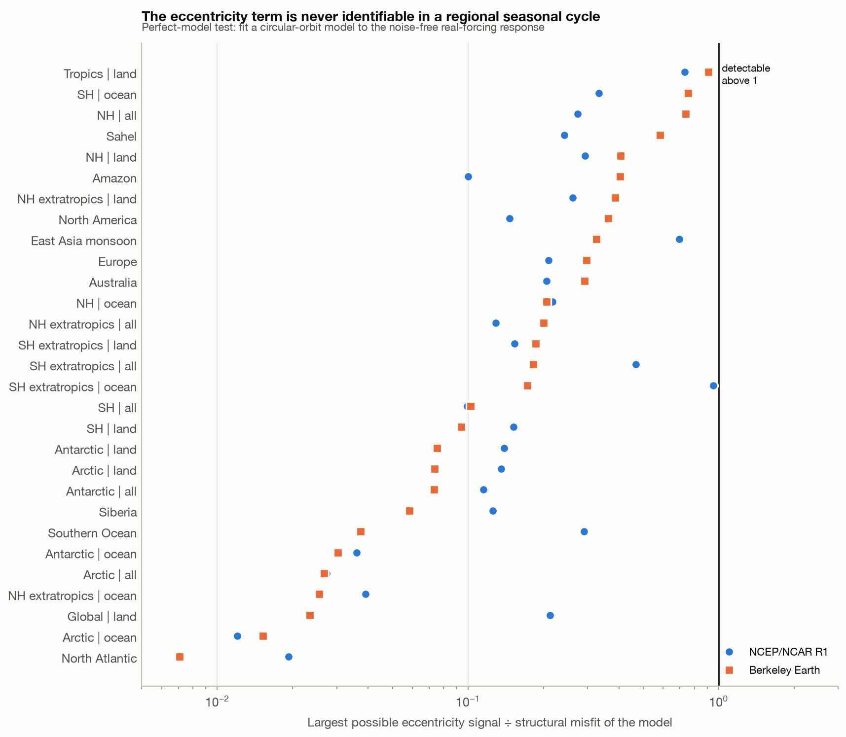
The eccentricity–precession part of the seasonal forcing cannot be identified in the response in any of 29 physically admissible regions at monthly resolution.
Global-mean temperature is anti-correlated (r = −0.95) with the global-mean insolation cycle, which is purely eccentricity-driven, and an unconstrained fit "explains" it with a negative gain.
A counterfactual circular orbit fits the tropical-land seasonal cycle better than the real orbit does.

Orbital time scales (0–2000 ka).

Precession pacing survives on a uranium–thorium dated speleothem chronology (coherence 0.98 at 23 kyr), and obliquity pacing survives in an ice core.
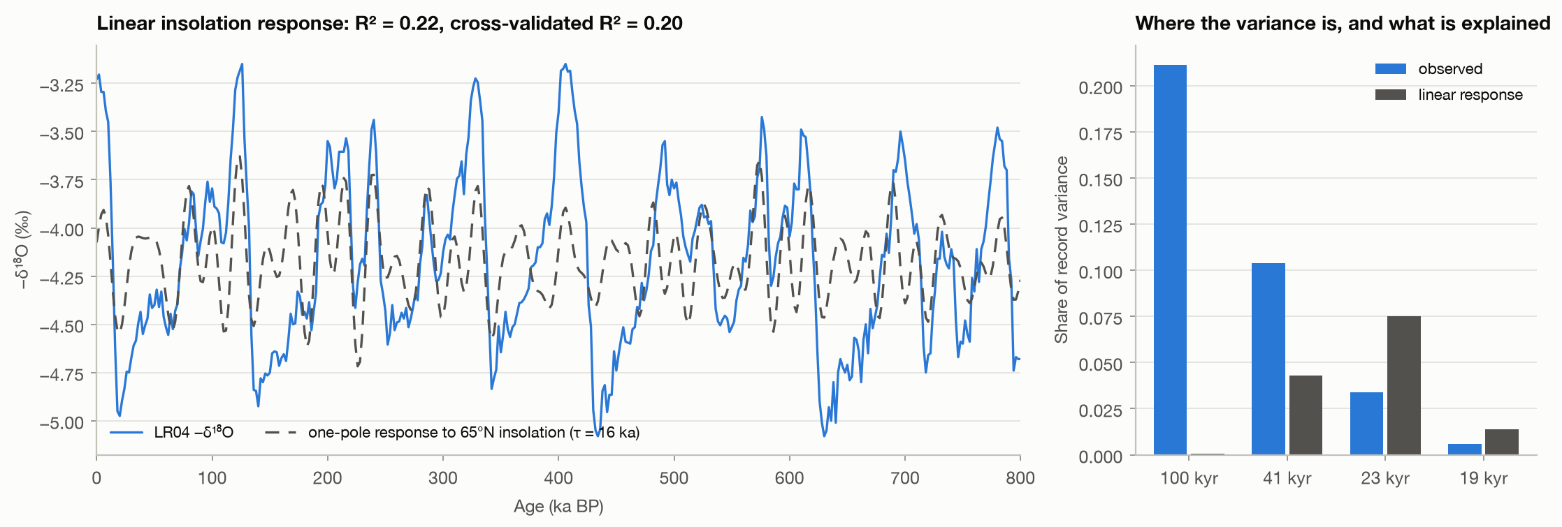
The 100-kyr cycle passes neither test. It is not coherent with eccentricity under a record-surrogate null (p = 0.054), and a linear insolation response reproduces 0.1% of the benthic stack's variance in that band against the 21% observed.
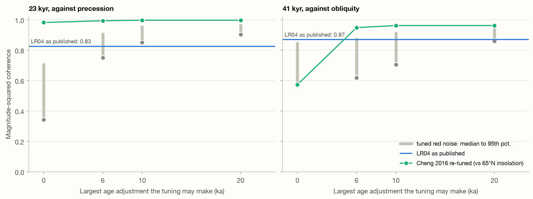
Aligning red noise to the forcing by dynamic time warping, with ±10 ka of freedom, produces precession coherence at the level published for the orbitally tuned LR04 stack.
On smoothed pure noise, a naive red-noise test finds a 100-kyr peak 44% of the time.

Across both regimes, predictive skill does not discriminate between mechanisms; transfer to forcing a model has not seen does.

Introduction

The seasons are orbital forcing made visible. Obliquity sets how far the Sun's declination swings through the year. Eccentricity and the precession of the equinoxes set how the Earth–Sun distance, and the orbital speed, vary against that swing. On time scales of 10⁴–10⁵ years the same three quantities change, and the Milankovitch hypothesis attributes the Pleistocene glacial cycles to the resulting redistribution of summer insolation (Hays et al. 1976; Imbrie et al. 1984; Berger 1978; Laskar et al. 2004).

The question "how much climate variability does orbital forcing explain?" therefore has two quite different forms, and this study treats them separately:

Regime A, the modern seasonal cycle. Over the instrumental era the orbital elements are effectively fixed, and orbital forcing is the seasonal cycle of insolation. Explaining the seasonal cycle of temperature is easy in the statistical sense, because almost any sinusoid fits it. The informative content lies elsewhere. How is the response lagged and damped? Does the forcing's finer structure appear in the response: the semiannual harmonic near the equator, and the asymmetry between hemispheres that comes from perihelion falling in January? And does a physically constrained model do anything a descriptive one cannot?
Regime B, the orbital cycles. Over 0–2000 ka the elements themselves vary. The classical evidence here is spectral: power in proxy records near 100, 41 and 23 kyr, and coherence with the orbital elements. That evidence has three well-known weaknesses. The periods are close on a log-frequency axis, every record is red, and the most-used chronology (LR04; Lisiecki and Raymo 2005) was built by aligning the record to 65°N insolation, the very forcing it is then tested against.

Throughout, we distinguish a predictive association (a model with orbital inputs forecasts the record) from a physical attribution (the association arises through a mechanism the forcing actually has). Most of the results below are cases where the two come apart.

Contributions.

A validated, reproducible insolation pipeline with two independent solar-position paths and a browser port checked against them.
A physically admissible response model for the seasonal cycle, and a perfect-model test for whether the eccentricity term is identifiable in climate at all.
A coherence null based on record surrogates, and a tuning-artefact null that measures how much orbital coherence alignment alone manufactures.
A model comparison in which transfer, not skill, separates physical from descriptive models.
A 2939-row robustness grid.

Data

Dataset	Variable	As distributed	Resolution	Chronology
La2004 (Laskar et al. 2004)	e, ε, ϖ	dimensionless; rad	1 kyr	astronomical
NCEP/NCAR R1 (Kalnay et al. 1996)	2 m air temperature; surface downward shortwave	degK; W m⁻²	monthly, T62 Gaussian	—
Berkeley Earth (Rohde and Hausfather 2020)	air temperature (anomaly + 1951–1980 climatology)	°C	monthly, 1°	—
LR04 (Lisiecki and Raymo 2005)	benthic δ¹⁸O	‰ VPDB	1–5 kyr	tuned to 65°N insolation
EPICA Dome C (Jouzel et al. 2007)	temperature anomaly	°C difference	~0.06 ka median	EDC3, glaciological with some orbital tie points
Cheng et al. (2016)	speleothem δ¹⁸O	‰ VPDB	~0.05 ka median	U–Th, untuned

Units are enforced, not assumed.

An absolute temperature outside 150–350 K stops the load. Berkeley absolute temperature is rebuilt from climatology plus anomaly before conversion.
Palaeo time is ka BP, positive into the past. La2004's negative kyr are negated on load, and the present-day elements (e = 0.01670, ε = 23.439°, ϖ = 102.92°) are asserted.
Area weights are exact spherical band areas, which reproduce the land fraction of the globe (0.284 and 0.288 against about 0.29).

LR04 is not uniformly sampled: 1 kyr to 600 ka, then 2, 2.5 and 5 kyr. It is therefore bin-averaged onto a uniform grid rather than treated as evenly spaced.

Orbital forcing and insolation

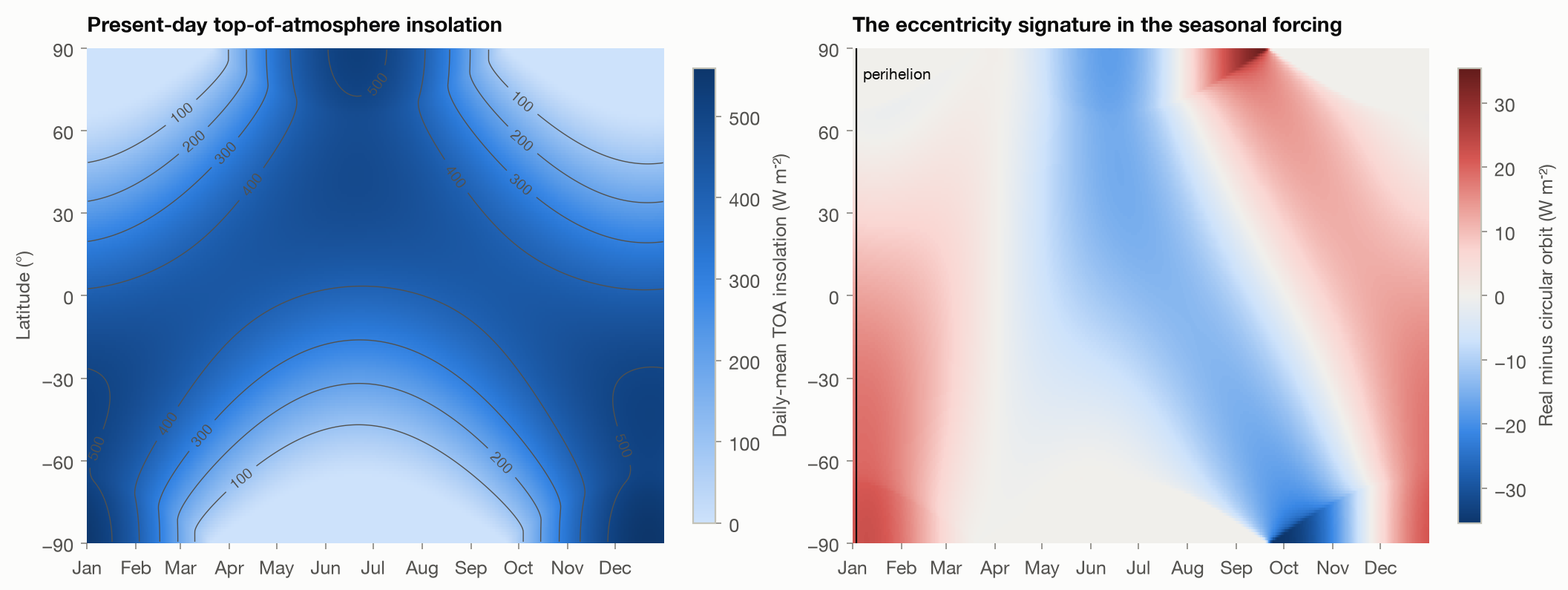
Daily-mean top-of-atmosphere insolation follows Berger (1978),

$\bar Q = \frac{S_0}{\pi}\left(\frac{a}{r}\right)^2\left[H_0\sin\phi\sin\delta + \cos\phi\cos\delta\sin H_0\right],\qquad \cos H_0 = -\tan\phi\tan\delta,$

with the polar-day and polar-night limits, $\sin\delta = \sin\varepsilon\sin\lambda$ , $a/r = (1 + e\cos\nu)/(1-e^2)$ and true anomaly $\nu = \lambda - (\varpi + \pi)$ . Here $S_0 = 1360.8$ W m⁻² (Kopp and Lean 2011). La2004's $\varpi$ is the heliocentric longitude of perihelion, so the Sun's apparent longitude at perihelion is $\varpi + \pi$ . A unit test pins this: an off-by-π error would move perihelion from early January to July.

The Sun's position is computed twice: from the Meeus (1998) solar theory on real dates, and from a Kepler solution driven by La2004 elements. The two agree to 0.018° over a year. The code reproduces:

the canonical present-day 65°N June-solstice insolation, 479.3 W m⁻² on the $S_0 = 1365$ convention (literature 479–481);
the closed-form global mean $S_0/(4\sqrt{1-e^2})$ to a relative error of 1.6e-06;
in its TypeScript port for the interactive site, the Python values to $10^{-12}$ W m⁻².

Present-day daily insolation (left) and its eccentricity–precession component: the real forcing minus a circular orbit with the same obliquity and equinox (right). The component combines the distance modulation, positive around perihelion, with the Kepler timing of the solstices and of the polar-day edges; the timing part produces the largest differences.

Methods

The seasonal cycle as a response to insolation

For each grid cell, zonal row and region we take the 1981–2010 monthly climatology and fit the one-pole relaxation

$C\frac{dT}{dt} = k'Q(t) - \lambda\,(T - T_0)\quad\Longrightarrow\quad \hat T(\omega) = \frac{k\,\hat Q(\omega)}{1 + i\omega\tau},\qquad \tau = C/\lambda.$

The daily insolation cycle is filtered in Fourier space and then averaged into calendar months, so monthly averaging is treated exactly. For fixed τ the model is linear, which makes the fit an exact profile over 174 values of τ. The primary fit is restricted to physically admissible parameters, $k \ge 0$ and τ ≤ 365 days. An unconstrained fit is retained only as a diagnostic, and in the tropics it wins only with a negative gain or a decade-long τ. The model has three parameters, as many as a one-harmonic regression, but it can only lag and damp the real forcing, harmonics included.

The seasonal share of monthly variance is computed within the baseline years. There the month-dummy projection makes the seasonal and anomaly parts exactly orthogonal, so the share of all monthly variance a seasonal model explains is exactly the seasonal share × R².

Eccentricity detectability. A free gain and lag absorb most of the eccentricity term, which is close to an annual harmonic peaking at perihelion, so a p-value on the improvement in R² answers the wrong question. The test instead has three steps:

Fit a circular-orbit model to the noise-free response of the real-forcing model.
Take its misfit, the most R² eccentricity could ever add.
Divide it by the real-forcing model's misfit to the data.

A ratio above 1 is the minimum condition for identifiability. Year-resampling bootstraps (B = 500) give intervals.

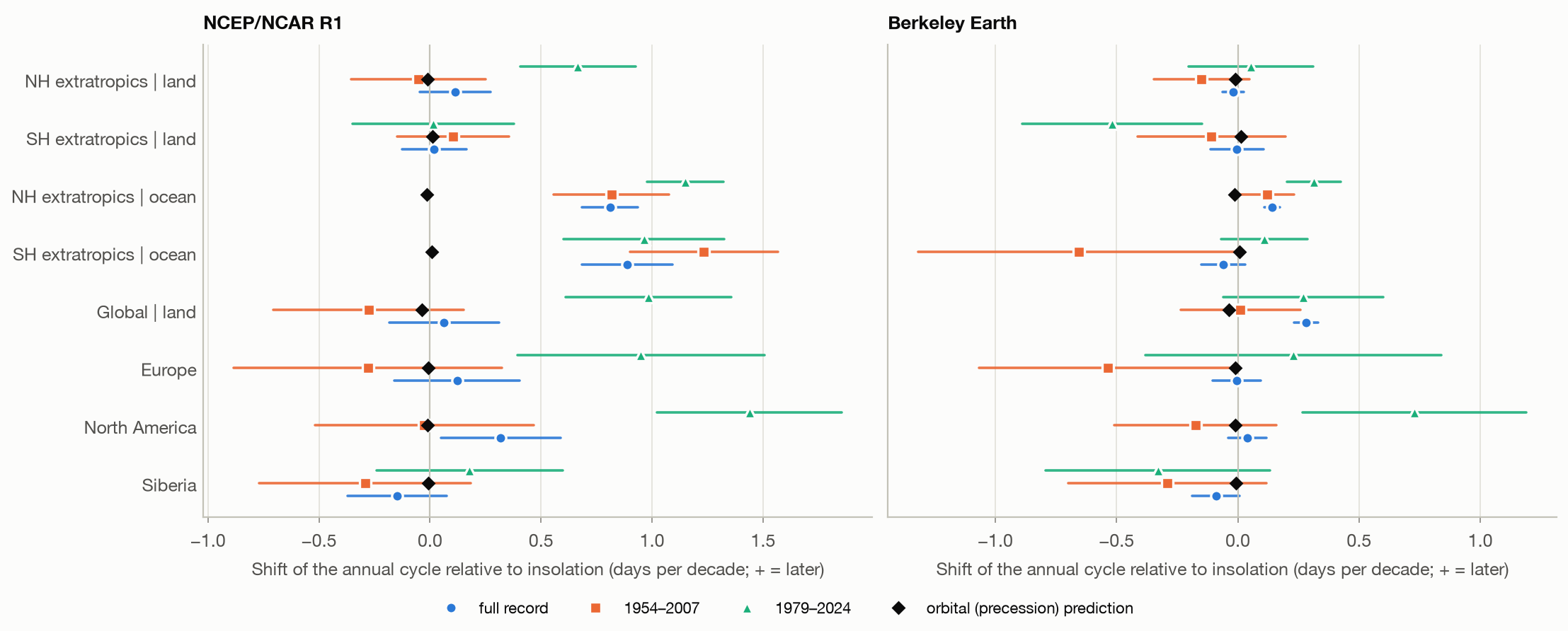
Seasonal timing. The day on which the annual harmonic peaks is computed per year and regressed on year with Newey–West (HAC) errors. It is measured relative to calendar-anchored insolation, because the Gregorian calendar's leap-year drift of the equinox (about −0.07 days per decade) would otherwise contaminate any calendar-based trend.

Orbital time scales

Gridding and windows. Records are bin-averaged onto a regular 2 ka grid. Three windows are used:

0–640 ka for all three records, giving the same length and estimator for the circularity comparison;
0–800 ka for LR04 and EPICA;
1250–2000 ka for LR04 before the mid-Pleistocene transition.

Spectra and band enrichment. Spectra are Thomson multitaper with NW = 3 (2.5 on the shorter window). The half-bandwidth $W = NW/(N\Delta t)$ decides whether the 23- and 19-kyr lines can be separated. At NW = 4 over 800 kyr they cannot, and every result reports its resolution. Band enrichment is the observed share of power in a band over the median share for 1000 fitted AR(1) surrogates.

Coherence. The null phase-randomises the record, not the forcing. The analytic multitaper coherence level assumes the tested series is locally white, and a record with its own spectral line at the forcing period violates that: two lines at one frequency are coherent whatever their phase. A unit test shows the analytic level then rejects almost always while record surrogates hold their size. Claims are restricted to physically meaningful pairs and corrected by Benjamini–Hochberg within each record.

The tuning-artefact null. Phase-randomised surrogates of LR04 keep its spectrum but carry no orbital phase. Each is aligned to a 65°N-insolation target (a one-pole response with τ = 15 ka) by slope-constrained dynamic time warping. Sedimentation-rate changes are limited to between ×0.5 and ×2, and total age adjustments to 0, 6, 10 or 20 ka. The untuned speleothem record is re-tuned the same way. Warping is more aggressive than LR04's tie-point procedure, so these numbers are upper bounds for a given age freedom.

Linear response. An insolation series is filtered by a one-pole relaxation in physical time, with τ chosen by blocked cross-validation (five blocks, 10 ka embargo). A surrogate R² null re-fits every τ for each of 500 phase-randomised copies of the record, so the freedom to pick τ is paid for.

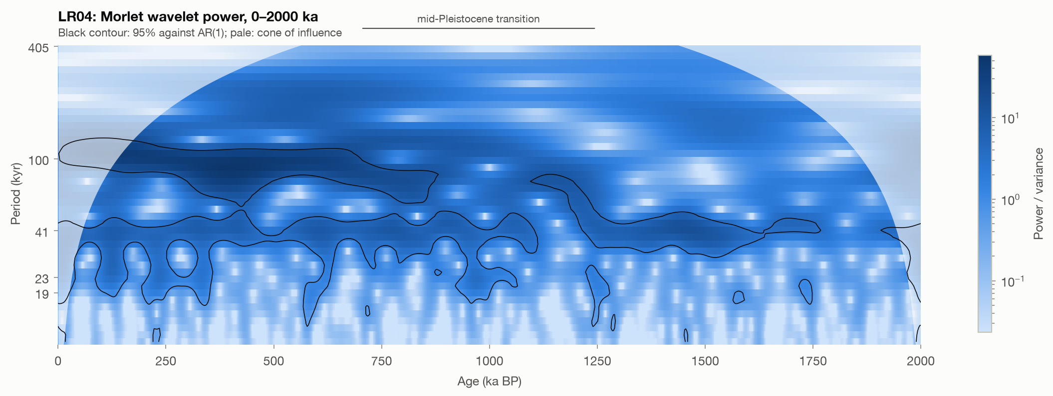
Wavelets. Morlet wavelets (Torrence and Compo 1998) are used only where non-stationarity is the question.

Model comparison, robustness and dependence

Model families. Eleven seasonal and seven orbital-scale models fall into three families:

physical: zero-lag and one-pole insolation responses;
statistical: climatology, harmonic and Fourier regressions, sinusoids at orbital periods, regression on orbital elements;
flexible: a Gaussian process on time and gradient boosting.

Evaluation. All share folds and metrics: blocked cross-validation with an embargo, an extrapolation split, and, for the seasonal cycle, transfer to latitude bands and domains the model never saw. Skill is the MSE improvement over a reference refitted on each training fold. Neural forecasting was deliberately not run. A three-parameter model already reaches the seasonal ceiling, and orbital inputs carry no year-to-year information for a network to learn.

Robustness. The grid varies temporal aggregation, baseline period, variable and dataset, which orbital terms are allowed, detrending, resampling step, multitaper bandwidth, predictor subsets, smoothing (with a naive and a smoothing-aware null) and random age-model error.

Dependence. Correlations use the Bretherton et al. (1999) effective sample size, which reduces the false-positive rate for independent AR(1) pairs with φ = 0.9 from 49.7% to 4.3%. Regressions use HAC errors. No inference counts grid cells. The monthly anomaly field has about 26 effective spatial degrees of freedom among 64778 valid Berkeley cells, and 36 among 18048 NCEP cells (Bretherton et al. 1999). The seasonal cycle itself has barely more than one.

Results

Most monthly variance is seasonal, and most of it looks like a response to sunlight

The seasonal climatology carries 83.1% of area-weighted monthly temperature variance in Berkeley Earth and 82.8% in NCEP. That is the ceiling for any purely seasonal model, and so for any model driven only by present-day orbital forcing.

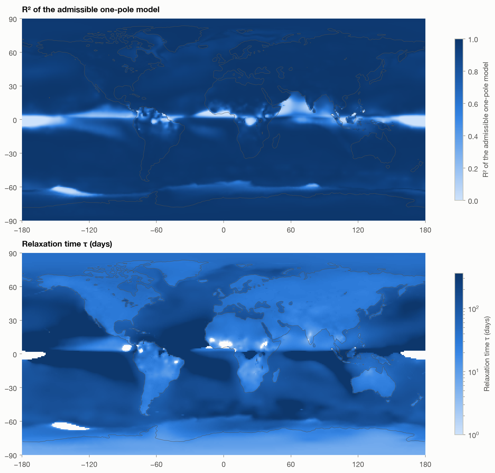
The admissible one-pole model reaches area-mean R² 0.912 on the seasonal cycle (NCEP 0.896), so it explains 78.1% (NCEP 76.3%) of all monthly variance.

The zero-lag insolation model reaches only 0.338. The lag is most of the physics: the relaxation time separates land from ocean at every latitude. Medians are 27 against 126 days in Berkeley, and 22 against 96 in NCEP. Heat capacity, not forcing, sets the difference.

In the single-region pilot run before any global analysis (NCEP land, 40–50°N), τ = 28.9 days implies an annual lag of 26.8 days, against 26.7 days measured directly from the data.

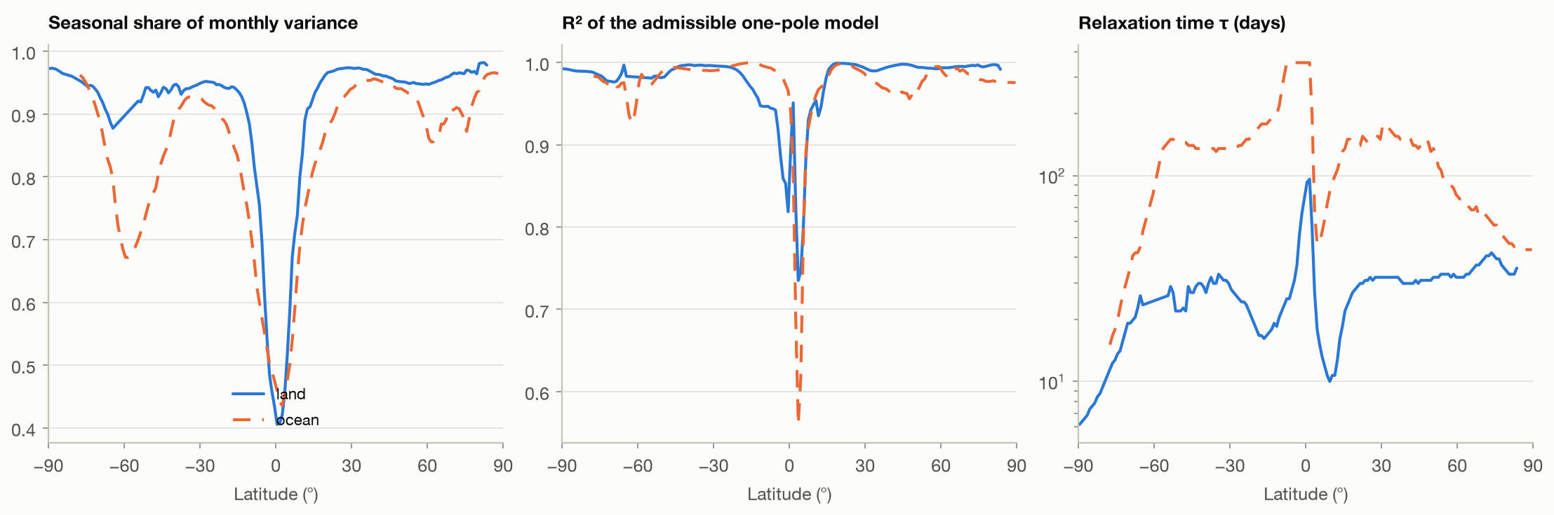
Zonal diagnostics (Berkeley Earth). The one-pole model fits the extratropical seasonal cycle almost perfectly and fails in the tropics; τ separates land from ocean.

The model fails where the seasonal cycle is not a local response to insolation: the equatorial Pacific cold tongue, and monsoon and rainforest regions. There the unconstrained fit is inadmissible over 14% of the globe's area, almost all of it tropical ocean.

The two datasets agree on the global picture but not everywhere. The Amazon's seasonal cycle is fitted with R² 0.47 in NCEP and 0.93 in Berkeley, a reminder that reanalysis 2 m temperature is strongly model-influenced in the tropics.

Does the forcing's finer structure survive? Where the insolation cycle has a strong semiannual harmonic, temperature has one too. The ratio of semiannual to annual amplitude is 0.32 in the Sahel, against 0.31 in its insolation and 0.27 in the one-pole response. In tropical land it is 1.92, against 1.81 in insolation; but the one-pole model explains little of that region's cycle, so the agreement is weak evidence there. In the extratropics the observed semiannual harmonic is several times what a response to insolation would carry: northern extratropical land 0.04 against 0.01, and the Southern Ocean 0.11 against 0.03. There the higher harmonics are set by something other than local insolation.

Cell-level R² and relaxation time (Berkeley Earth, 1°).

A better fit is not a better explanation

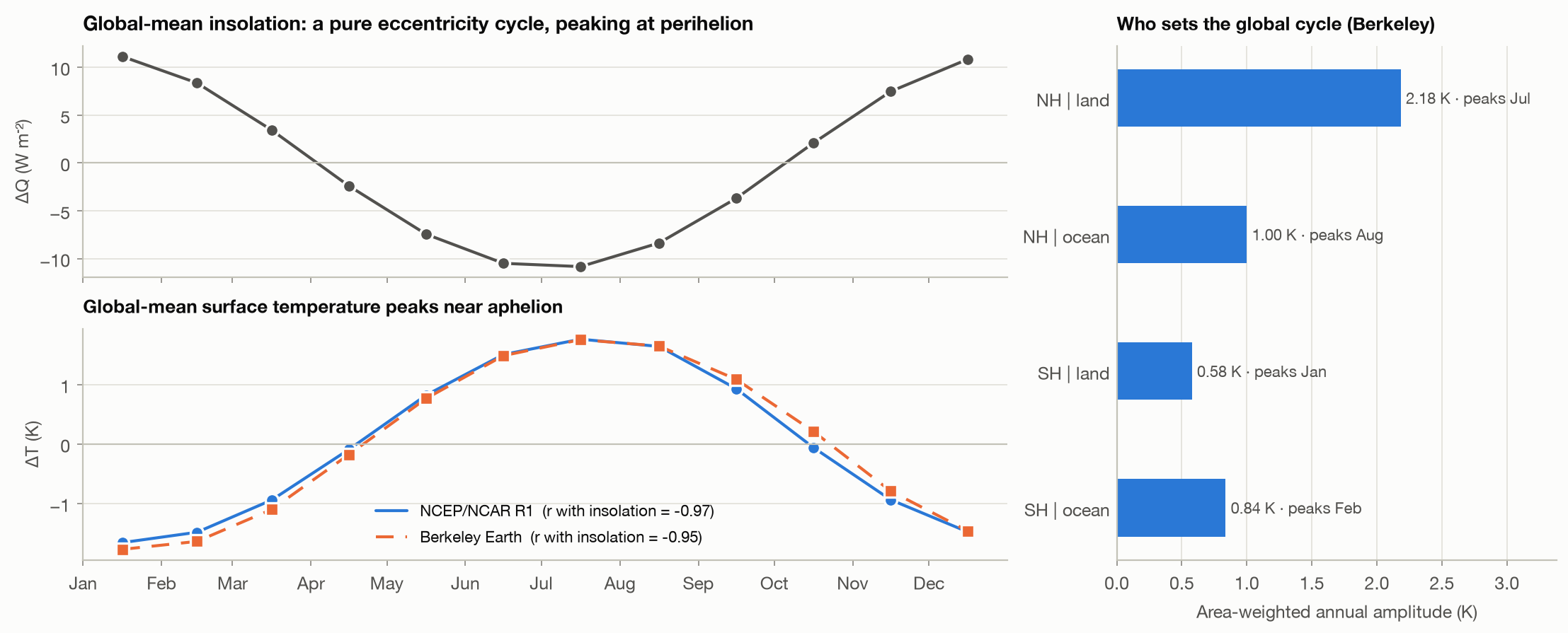
With a circular orbit the global-mean insolation would be constant through the year; the numerical standard deviation of the circular case is 0.001 W m⁻². The real global-mean insolation varies by 22.0 W m⁻² and peaks on day 3, at perihelion: the global-mean seasonal forcing is purely an eccentricity signal.

Global-mean surface temperature peaks on day 203 (NCEP 198), near aphelion. Over the 12 months it is correlated with the insolation at r = -0.954 (NCEP -0.974). The unconstrained response model "explains" the global cycle with R² = 0.999 using a gain of -0.17 K per W m⁻²: more sunlight, colder. The admissible model explains R² = 0.000.

The decomposition in the figure is the reason. Northern-hemisphere land is a fifth of the globe with a small heat capacity, and it dominates the global annual harmonic and pins it to July. The land–sea asymmetry between hemispheres confounds the global relationship. The association is real and strong, and it is not attribution.

Global-mean insolation and temperature, and the area-weighted contributions to the global annual harmonic.

A counterfactual makes the same point regionally. In tropical land, a circular-orbit forcing with no eccentricity fits the seasonal cycle with R² 0.97, against 0.29 for the real forcing. In the southern extratropical ocean a forcing with no obliquity at all fits as well as the real one (R² 0.997). The southern summer solstice falls only days before perihelion, so the shape of the forcing cannot tell the two orbital terms apart; only the implied gain can.

Surface shortwave radiation behaves as expected of a direct radiative response. In NCEP it follows the global eccentricity cycle with r = 0.89 and τ ≈ 0 in the extratropics, while temperature is anti-correlated. That flux is model-only in the reanalysis, so it illustrates the mechanism rather than confirming it.

The eccentricity term is in the forcing, not identifiably in the response

The eccentricity–precession component of the seasonal forcing is not small: ±3.3% in distance modulation, plus a timing effect up to tens of W m⁻² at the polar-day edges. Yet at monthly resolution the most R² it could add is smaller than the real-forcing model's own misfit in every admissible region. That holds in all 29 Berkeley regions (median ratio 0.18, largest 0.91) and all 29 NCEP regions (median 0.15, largest 0.95).

Consistent with this, the circular-orbit forcing fits as well as or better than the real one over 41% of the area, a coin toss. The claim is scoped to monthly data. With seasonal means only one residual degree of freedom remains, R² reaches 1 and the ratio's denominator collapses (for example 3.26 for northern extratropical land), so values above 1 there are artefacts.

Eccentricity detectability for every physically admissible region, both datasets. No region reaches 1.

Modern changes in seasonal timing are not orbital

Precession moves the phase of the annual insolation cycle by at most 0.04 days per decade in any region (for northern extratropical land, -0.011). Measured against insolation, the annual temperature cycle over northern extratropical land shifted by -0.15 ± 0.10 days per decade over 1954–2007 in Berkeley (p = 0.14). That is the direction reported by Stine et al. (2009), but it is not significant once the calendar drift is removed.

Across windows and datasets the observed shifts change sign. Over the ocean, NCEP's large later-shifts (+0.81 days per decade) are not reproduced by Berkeley (+0.14). Orbital forcing cannot explain the observed changes, and the observed changes are not robust enough to attribute to anything with confidence from these data.

Trends in the timing of the annual temperature cycle relative to insolation, with the precession-only prediction.

Orbital periodicities, with a chronology that owes nothing to the orbit

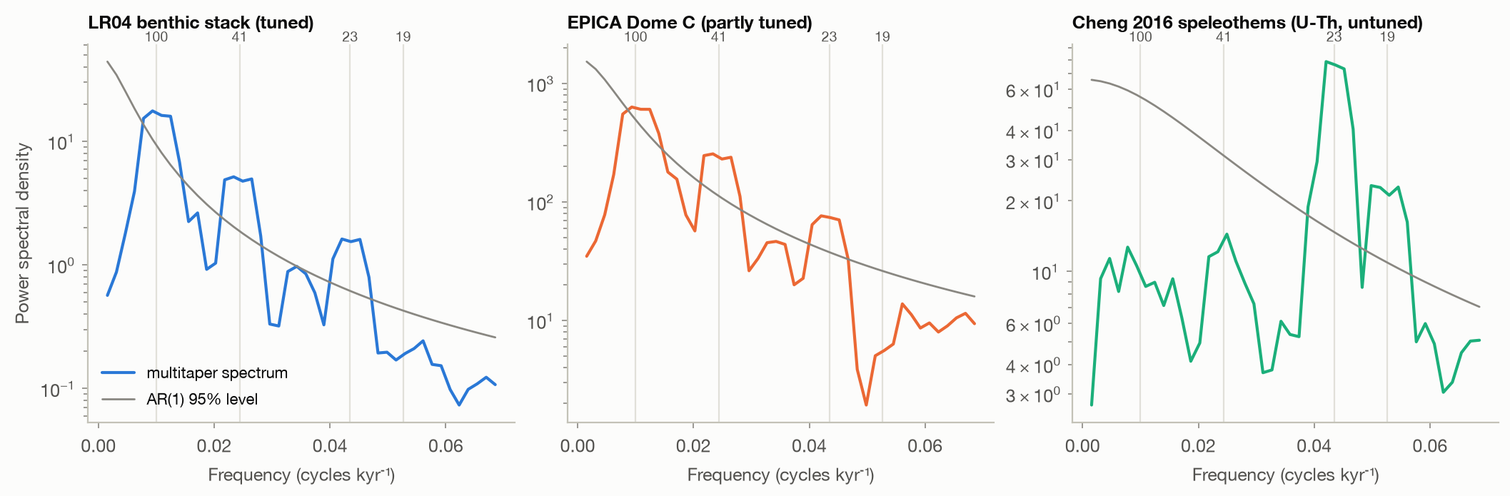
All three records carry excess power in orbital bands:

LR04 (0–800 ka) is enriched 4.6-fold at 41 kyr, 3.5-fold at 23 kyr and 2.5-fold at 100 kyr over a fitted AR(1).
The speleothem record is enriched only at 23 kyr (9.2-fold) and 19 kyr (3.9-fold).

Multitaper spectra on a common 0–640 ka window against an AR(1) 95% level.

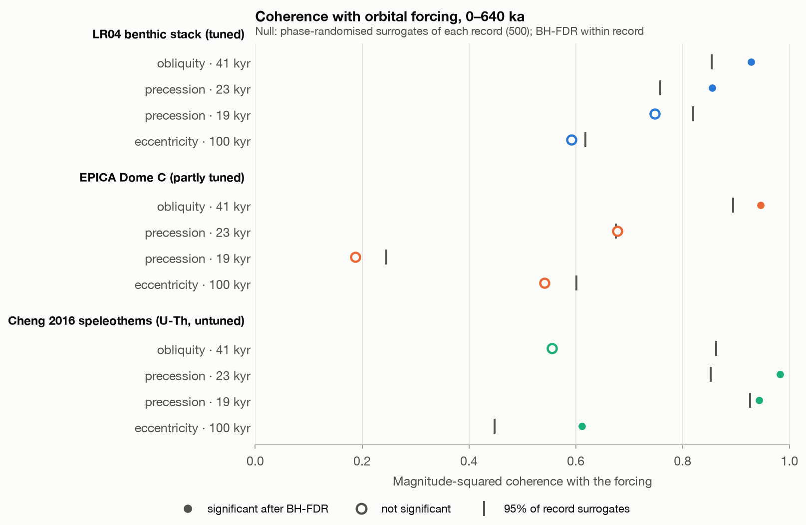
Coherence against record surrogates, after Benjamini–Hochberg correction.

LR04 is coherent with obliquity at 41 kyr (0.87, p = 0.028) and with precession at 23 kyr (0.83, p = 0.004). Its record lags the forcing by +6.4 and +4.1 ka. These lags are partly a property of the tuning target, not independent evidence.
EPICA is coherent with obliquity (0.92, p = 0.002) but not with precession (0.64, p = 0.118).
The decisive record is the one whose chronology owes nothing to the orbit. The U–Th dated speleothems are coherent with precession at 23 kyr (0.98, p = 0.002) and 19 kyr (0.94, p = 0.030). They lag June-solstice insolation by only +2.6 ± 0.2 ka, which is close to in phase with mid-July insolation.

Precession pacing of the Asian monsoon is therefore not an artefact of tuning.

The 100-kyr cycle is where the evidence fails. LR04's coherence with eccentricity at 100 kyr (0.69) does not beat its record surrogates (p = 0.054), and EPICA's does not either.

Before the mid-Pleistocene transition LR04 is dominated by a clean 41-kyr cycle (enrichment 7.0-fold), yet its obliquity coherence (0.84) fails correction. This is a limit of coherence, not evidence against pacing. A single line is coherent with any sinusoid of its period, so record surrogates that keep the line reach similar coherence; band enrichment is the relevant evidence there.

Coherence with the orbital elements on a common window; filled points survive Benjamini–Hochberg correction against record surrogates.

Tuning, smoothing and age error manufacture or destroy the evidence

LR04's published precession coherence is 0.83. Red noise with LR04's spectrum reaches a median of 0.75 at 23 kyr once tuned with ±6 ka of freedom, 0.85 with ±10 ka, and 0.90 with ±20 ka. Re-tuning the untuned speleothem record by ±6 ka raises its 41-kyr coherence with 65°N insolation from 0.57 to 0.95, although that record has no enriched 41-kyr power. Coherence at these levels is therefore not evidence of pacing in a tuned record unless the tuning's age freedom was well below about 6 ka.

Coherence manufactured by tuning red noise with LR04's spectrum, as a function of the age adjustment the tuning may make.

Smoothing. On pure AR(1) noise matched to LR04, a naive red-noise test applied after a 40-ka running mean flags the 100-kyr band in 44% of replicates. A 10-ka mean flags the 41-kyr band in 31%. A smoothing-aware null, which fits the AR(1) to the raw series and smooths every surrogate identically, stays at or below 4%. On the real records the naive test both fabricates peaks and erases real ones.

Age error. Adding smooth random age error to each chronology shows how fragile precession coherence is. LR04's 23-kyr coherence stays significant in 90% of draws at 2 ka standard deviation, 40% at 4 ka and 7.5% at 6 ka. For the speleothems it survives in only 32% of draws even at 2 ka. Precession coherence as high as observed requires a chronology accurate to well under ~2 ka, or one that was aligned to the forcing.

How much orbital-scale variance is a linear response to insolation

The best linear response of LR04 to 65°N insolation (τ = 16 ka) explains R² = 0.22 (cross-validated 0.20; surrogate p = 0.002). A regression on all four orbital elements reaches 0.34. The linear insolation response reproduces the 41- and 23-kyr structure but carries 0.1% of the record's variance in the 100-kyr band, against 21% observed. This is the 100-kyr problem restated as a variance budget: the forcing has almost no power where the response has the most.

The wavelet transform locates the change. The ratio of 100- to 41-kyr power is 4.29 over 0–700 ka and 0.15 over 1250–2000 ka, while the forcing did not change character.

The best linear response of LR04 to 65°N insolation, and the variance it explains in each orbital band.

Wavelet power of LR04 across the mid-Pleistocene transition.

The monsoon record is the one well explained by a physical linear response. Local (30°N) summer insolation explains R² = 0.54, cross-validated 0.54. EPICA's linear orbital signal is carried by obliquity (cross-validated R² 0.173) rather than precession (0.009). Its local southern summer insolation performs worst (-0.001), because its precession component is out of phase with the record's weak precession signal. We therefore do not read EPICA's better fit to northern insolation as evidence that Antarctic temperature follows the north.

Prediction and transfer rank models differently

Seasonal regime. Every model hits the same ceiling, the monthly climatology, because in the modern era orbital inputs are a calendar. Out of sample the three-parameter physical model is slightly worse than twelve monthly means. In northern extratropical land, cross-validated R² is 0.989 against 0.991, which is a skill of -0.151 relative to climatology on the anomaly scale.

A Gaussian process on time achieves the best cross-validated skill (+0.592 in the same region) by interpolating the warming trend inside held-out blocks. It does not extrapolate: trained on 1948–1985 and tested on 1990–2024, its skill in NCEP's northern extratropical land is -3.523.

Gradient boosting given only orbital inputs beats climatology in tropical land, with cross-validated skill +0.533 (Berkeley). The reason is not physical. A calendar month's mean insolation drifts slightly from year to year, through Gregorian leap-year drift of the equinox and through precession: by up to 0.0601 W m⁻² per decade in that region, and in step with the year. A tree ensemble can use that drift as a clock for the warming trend. Replacing each month's insolation by its climatological value, identical every year, reduces the skill to +0.000, as it does in every region and dataset tested. Where weather noise dominates, as in northern extratropical land, the clock does not even help (-0.479 in NCEP). An orbital-input model with skill beyond climatology is therefore not, by that fact, evidence of orbital influence on anomalies.

Transfer separates the families. One τ and gain shared across northern land predict the seasonal cycle of whole 10° latitude bands held out of training with R² 0.992. The mean training cycle, the best a forcing-free description can transfer, reaches 0.913, and zero-lag insolation 0.761.

Transfer across domains fails for every model. Northern land learns τ = 32 days, while the northern ocean would choose 106. Southern land wants a gain less than half of northern land's. The one-pole parameters are properties of a surface and a hemisphere, not universal constants.

Orbital regime. Free sinusoids at the La2004 periods beat the physical insolation response for LR04: cross-validated R² 0.33 against 0.19. They win by fitting the 100-kyr band with free amplitude, the band no linear insolation pathway can produce, so predictive association again outperforms a physical account. A Gaussian process on age cannot extrapolate between the younger and older halves at all.

Robustness

Axis	What changes	What does not
Baseline period (1951–1980 … 1991–2020, full)	Ocean τ by ±10 days; seasonal share in long windows (trend)	Land τ (28.9 d in NCEP under all four), R², admissibility
Dataset (NCEP vs Berkeley)	Tropical land and Amazon fits; ocean phase trends	Seasonal share, eccentricity result, global anti-phase
Temporal aggregation	Detectability ratio (meaningless at 1 residual dof)	Monthly conclusions
Orbital terms allowed	Tropical land prefers a circular orbit; SH ocean cannot tell the terms apart	Extratropical land requires obliquity
Detrending	Tropical-land seasonal share (0.67 → 0.86, Berkeley)	Extratropical shares
Resampling step, detrending (Regime B)	—	Band enrichment, coherence, linear-response R²
Multitaper bandwidth	p-values near 0.05 (LR04 precession at NW ≤ 2.5); resolution of 23/19 kyr	Obliquity and speleothem precession significance
Smoothing	Naive tests (fabricated and erased peaks)	Smoothing-aware tests
Age error	Precession coherence collapses for σ ≳ 2–4 ka	Obliquity coherence degrades more slowly

Reviewer 2: the case against this paper

"The physics is a cartoon." Yes: a one-pole relaxation per cell, with no advection, no hydrology and no sea ice. We use it because it is the minimal model that can only produce filtered copies of the real forcing, so where it fits, the forcing's shape is sufficient, and where it fails, something else sets the cycle. It fails exactly where one would expect (the tropics, monsoons, the cold tongue). We do not interpret its gain as a climate sensitivity, and we never extend it to the orbital regime beyond a linear-response baseline.

"Everything is confounded with time." In the modern era, temporal confounding enters three ways, and each is handled explicitly.

The warming trend. It is reported through detrending sensitivity and by separating seasonal from anomaly variance within baseline years.
Calendar drift. It is removed by measuring phase relative to calendar-anchored insolation, and shown to leak into flexible models as a clock.
The land–sea configuration. It makes the global mean anti-phased with its forcing, and it is the reason no global-mean statement is made about attribution.

In the palaeo regime, time is confounded with the chronology itself, which is why the untuned record and the tuning null exist.

"Your p-values ignore autocorrelation." They do not. Correlations use effective sample sizes, regressions HAC errors, spectra AR(1) nulls fitted to each record, coherence phase-randomised record surrogates, and linear-response R² a surrogate null that re-selects τ every time. The smoothing experiment shows what happens when the red-noise null is mis-specified.

"A map with 64,800 cells has 64,800 chances to look significant." No inference counts cells. The Berkeley anomaly field has about 26 effective spatial degrees of freedom. Maps and area fractions are descriptive, and regional statements are made on 34 pre-specified aggregates with bootstrap intervals.

"Your models will not extrapolate." Correct, and measured. The Gaussian process wins cross-validation and loses badly in extrapolation. Cross-domain transfer fails for every model. Palaeo models are tested across the halves of each record, and nothing here is extrapolated to future orbital configurations.

"You say 'explains' when you mean 'fits'." Throughout, "explains R²" means a fraction of variance fitted or predicted. Attribution statements are confined to cases where the forcing's physics and a counterfactual forcing agree. We state explicitly where fits are not attribution: the global mean, tropical land, the 100-kyr band, flexible models with orbital inputs, and tuned coherence.

Discussion and limitations

The seasonal cycle is where orbital forcing is strongest, and it is also where statistical explanation is least informative. Any seasonal model reaches the same ceiling, so skill cannot distinguish a physical account from a description; only transfer and counterfactual forcings can. On orbital time scales the evidence is strongest where the chronology is independent of the forcing (precession in the monsoon) and weakest where the dominant variance lies (the 100-kyr cycle). That is consistent with a nonlinear ice-sheet response to insolation pacing (Imbrie et al. 1984; Huybers 2006), which a linear framework can detect only as unexplained variance.

Limitations:

No climate model or intervention.
NCEP temperature is model-influenced and its surface shortwave model-only.
The tuning null uses dynamic time warping, which is more aggressive than LR04's procedure.
Age errors are modelled as stationary.
The orbital-scale analysis is linear by design.
The detectability ratio uses the one-pole model's structural misfit as its yardstick; a more complete physical model with smaller misfit could, in principle, make the eccentricity term identifiable in some regions.

Conclusion

Orbital forcing, through the seasonal cycle of sunlight, accounts for most monthly temperature variance on Earth. A one-pole response with one timescale per surface captures it and transfers across latitudes within a surface type. But the fit does not identify which orbital terms matter, and the global-mean cycle runs opposite to its own forcing. On orbital time scales, precession and obliquity pacing survive tests designed to break them, while the 100-kyr cycle does not survive as a linear response. Tuning and smoothing can manufacture the evidence they are used to find. Across both regimes, the useful question is not whether a model with orbital inputs predicts well, but whether it predicts forcing it has never seen.

Data and code availability

All data are public; sources, versions and SHA-256 checksums are recorded in data/raw/MANIFEST.json and the site's methods page. The full pipeline (scripts/00–08) regenerates every table, figure and number. scripts/verify_claims.py checks each tagged number in this text against results/canonical_results.json. The test suite validates the orbital geometry against published values and the statistical machinery on synthetic series with known answers.

References

Berger, A. (1978). Long-term variations of daily insolation and Quaternary climatic changes. Journal of the Atmospheric Sciences 35, 2362–2367.
Bretherton, C. S., Widmann, M., Dymnikov, V. P., Wallace, J. M. and Bladé, I. (1999). The effective number of spatial degrees of freedom of a time-varying field. Journal of Climate 12, 1990–2009.
Cheng, H. et al. (2016). The Asian monsoon over the past 640,000 years and ice age terminations. Nature 534, 640–646.
Hays, J. D., Imbrie, J. and Shackleton, N. J. (1976). Variations in the Earth's orbit: pacemaker of the ice ages. Science 194, 1121–1132.
Huybers, P. (2006). Early Pleistocene glacial cycles and the integrated summer insolation forcing. Science 313, 508–511.
Imbrie, J. et al. (1984). The orbital theory of Pleistocene climate: support from a revised chronology of the marine δ¹⁸O record. In Milankovitch and Climate, Part 1, 269–305. Reidel.
Jouzel, J. et al. (2007). Orbital and millennial Antarctic climate variability over the past 800,000 years. Science 317, 793–796.
Kalnay, E. et al. (1996). The NCEP/NCAR 40-year reanalysis project. Bulletin of the American Meteorological Society 77, 437–471.
Kopp, G. and Lean, J. L. (2011). A new, lower value of total solar irradiance: evidence and climate significance. Geophysical Research Letters 38, L01706.
Laskar, J., Robutel, P., Joutel, F., Gastineau, M., Correia, A. C. M. and Levrard, B. (2004). A long-term numerical solution for the insolation quantities of the Earth. Astronomy & Astrophysics 428, 261–285.
Lisiecki, L. E. and Raymo, M. E. (2005). A Pliocene–Pleistocene stack of 57 globally distributed benthic δ¹⁸O records. Paleoceanography 20, PA1003.
Meeus, J. (1998). Astronomical Algorithms, 2nd edition. Willmann-Bell.
Rohde, R. A. and Hausfather, Z. (2020). The Berkeley Earth land/ocean temperature record. Earth System Science Data 12, 3469–3479.
Stine, A. R., Huybers, P. and Fung, I. Y. (2009). Changes in the phase of the annual cycle of surface temperature. Nature 457, 435–440.
Torrence, C. and Compo, G. P. (1998). A practical guide to wavelet analysis. Bulletin of the American Meteorological Society 79, 61–78.